For the first part of this post I invite you to take a look at my friend Satyajit’s post where he describes the data layout of OSM and talks about rendering it in matplotlib.
Starting point
In this post I shall describe the technique used to render the OSM data in an OpenGL environment and some performance improvements that were conducted.
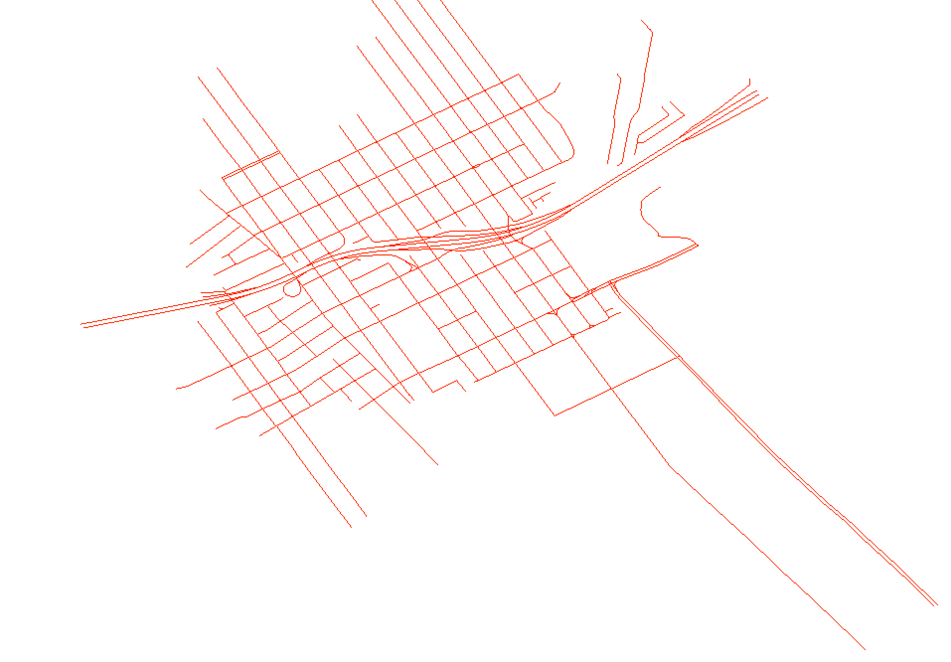
First, this is what was is obtained if vispy’s data is rendered as is:

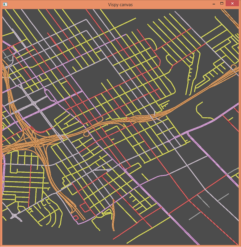
And finally we were able to obtain the following image:

Why is this a problem?
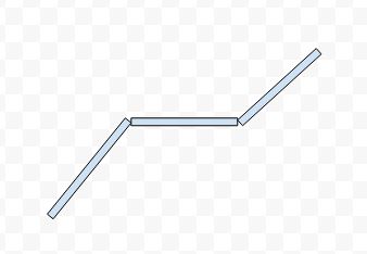
At first glance it’d seem that the easiest way to render a thick line when we have a thin one is to increase the line thickness. This mostly works but there is something unappealing about the result. It looks as if a child has abruptly stacked some rail road tracks end to end without taking the time to join them. I no longer have images to show how they looked but the following diagram is a good approximation.
The rotated rectangle approach
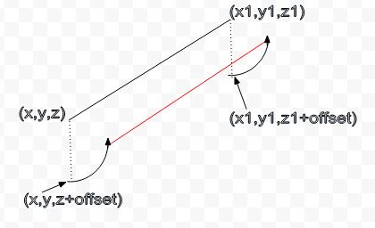
I think of this as rather like a door. Say the coordinates of a line in a plane are (x, y, z) and (x1, y1, z1), we create two new points (x, y, z+offset) and (x1,y1, z1+offset). If you were to drop a plumb line from each of these points then the new points would have the same x and y coordinates but the z value would change by some amount.
Now join the original two points to get the equation of a line and using that line as an axis rotate the new points by 90 degrees. This will raise the new points to the z same level as the original points. In the figure below the line in red is what is obtained by joining the two new points obtained after rotation.
Performance issues
What about the perf issues with rotating? Since this implies multiplying a rotation matrix with each point.
This is indeed a valid point, however it can be mitigated somewhat by splitting the multiplication directly to get the x, y, and z components after rotation and then throwing away the calculations for Z since we know that after rotation it will be the same as the original z. Here is the code for the rotation:
def extrude_point(curX, curY, axisVector, scale):
    extrudedPoint = [curX, curY, scale, 1]
    rotatedExtrudedPoint = [0, 0, 0]
    axisVector = normalize_vec(axisVector)
    a = curX
    b = curY
    u = axisVector[0]
    v = axisVector[1]
    x = extrudedPoint[0]
    y = extrudedPoint[1]
    z = extrudedPoint[2]

    rotatedExtrudedPoint[0] = (a * v * v ) -  (u * ((b * v) - (u * x) - (v * y)) + (v * z))
    rotatedExtrudedPoint[1] = (b * u * u) - (v * ((a * u) - (u * x) - (v * y)) - (u * z))
    rotatedExtrudedPoint[2] = (a * v) - (b * u) - (v * x) + (u * y)
    return rotatedExtrudedPoint
In the above code segment the last set of multiplications to get rotatedExtrudedPoint[2] are unnecessary.
While this looks better, than the line width approach, on it’s own its not very useful, it still looks like rectangles stacked end to end.
Framerates
After adding in an index buffer when we measured the performance we got a miserable 4 fps. The reasons were quite obvious. We were rendering the data that came from OSM unmodified i.e if the data gave us twenty discrete sets of coordinates for twenty roads we would submit twenty draw calls.
The solution was therefore to merge this data into one VBO create an IBO for it and to submit 1 draw call. This yielded frame rates of about 62 fps.
One other advantage of merging the data into a single VBO is that no longer does it look as discrete rectangles stacked end to end.

